Fine-tuning ML Models with Hugging Face

A Walkthrough Using Hugging Face and TensorFlow APIs

Hugging Face is quickly becoming the GitHub of machine learning. Whereas GitHub provides a massive platform for open-source contributions for traditional software, Hugging Face is the platform for open-source, state-of-the-art machine learning models and datasets.

Using Hugging Face’s transformers and datasets libraries, we can quickly load a pre-trained model like BERT, T5, or GPT-2 (or variations like DistilBERT) and run inferences on our own specific tasks. This is important because machine learning is a highly iterative process where we try different models and hyperparameters and experiment to see what works best.

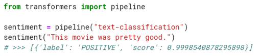
The fastest and easiest way to run a Hugging Face model is using the pipeline function – we can load a model and run predictions in only a few lines of code. For example, an entire (text) sentiment analysis workflow can be created like so:

However, for this article, we’ll look at how to fine-tune a pretrained model (for sentiment analysis). It requires more time and effort, but we will be rewarded with a better, more accurate model that’s tailored to our specific use case.

When we go to Hugging Face’s website, we see a listing of various machine learning models, and to the left, we can filter the list by domain/task, language, etc:

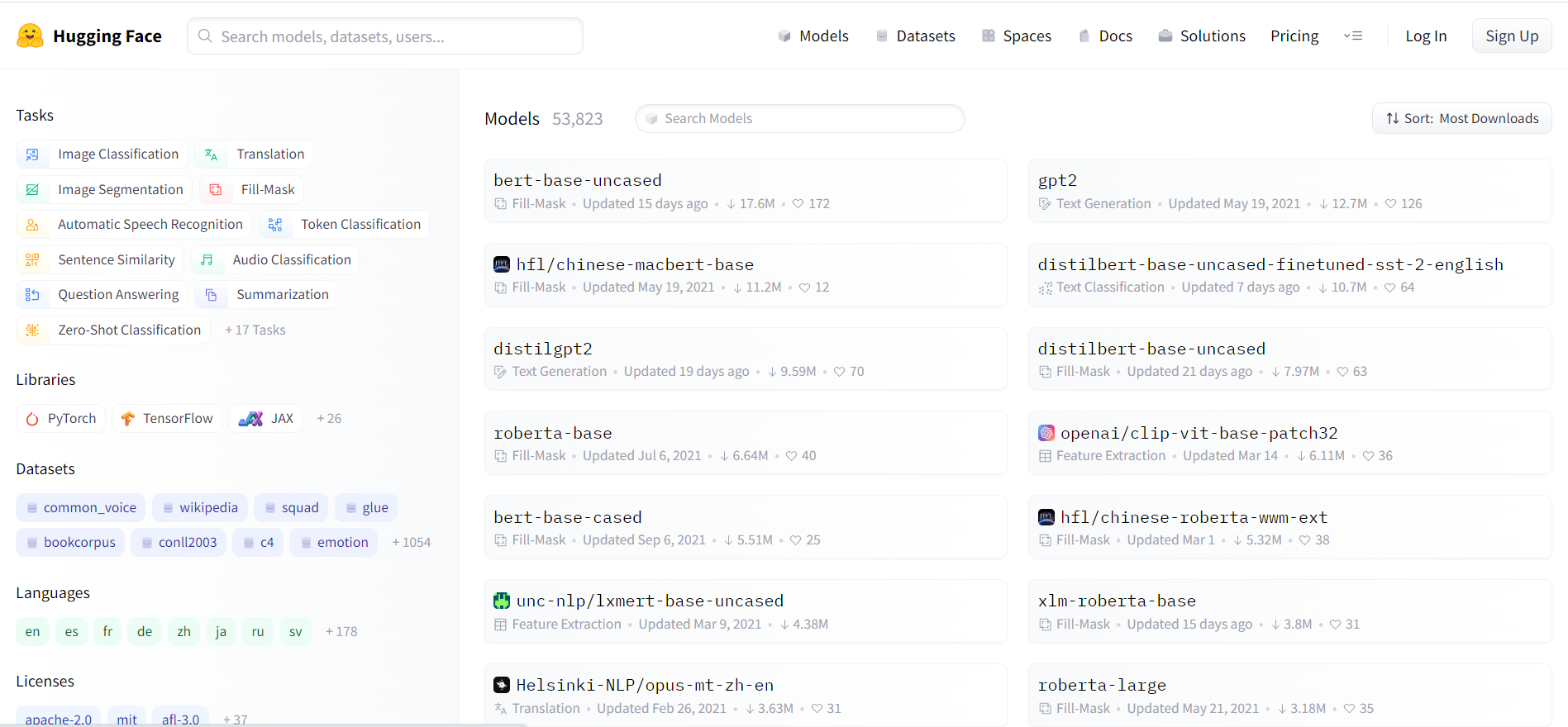
If we select one of the models, we can view detailed information about it. Since everything is handled through Hugging Face's libraries, we don’t need to clone a repo or download anything from the site – just copy the name of the desired model.

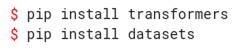
Let’s install the necessary packages. As usual, we should be using a virtual environment (venv, conda, etc.). With our virtual environment activated, we will install both the transformers and datasets packages with pip:

Fire up Jupyter Notebook and let’s start importing the requisite packages:

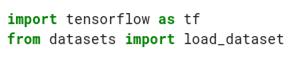
You’ll notice that we’ve imported TensorFlow in addition to datasets. If you’ve used TensorFlow (Keras) in the past, then much of the code we’re going to write will look familiar. That is because all of Hugging Face’s models are also Keras model objects; and therefore, have the same Keras API. (Hugging Face’s APIs support both TensorFlow and PyTorch, but I’ll be using TensorFlow for this article.)

Let’s load some data: we’ll be using the Amazon Fine Food Reviews dataset. In general, the distribution of Amazon product reviews tends to be highly skewed: either lots of high scores and very few neutral and low scores; or lots of high and low scores, but very few neutral. We would need to resample the data to get a balanced dataset. Normally, when we work with data, we would want to explore and clean the data before we start working on our machine learning model. However, data cleaning is outside the scope of this article, so we will assume that the data we load in our notebook has already been cleaned, balanced, and transformed.

Hugging Face’s datasets is a high-performance data structure that allows large amounts of data to be read and/or processed efficiently. It also features a clean API, so we can load data with a single statement:

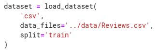
Here, we use the load_dataset() method, specifying the file type and file path. We also pass the optional split argument and specify that we want to create a training set. Subsequently, we split our data into train and test sets, allocating 1% of the data (rows) as the test set:

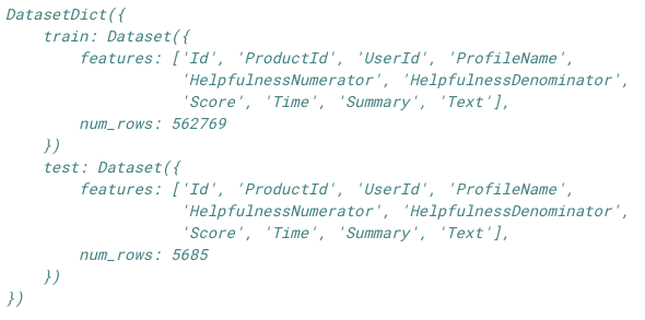
If we print out the dataset variable we just created, we will get something like this:

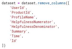
We can see that “train” and “test” are subsets of a DatasetDict object. We’re also provided information about the number of examples (“num_rows”) in each set and the column names (“features”) of the data. Since we’re trying to discern user sentiment of product reviews, we don’t need all of these columns, just the “Score,” which is an integer value based on Amazon’s 1–5-star rating system, and “Text,” which is the actual review text. As alluded to earlier, we should handle the feature engineering in earlier steps; however, Hugging Face datasets provides us with some useful tools to prepare our data. We can drop superfluous columns from our dataset with the .remove_columns() method:

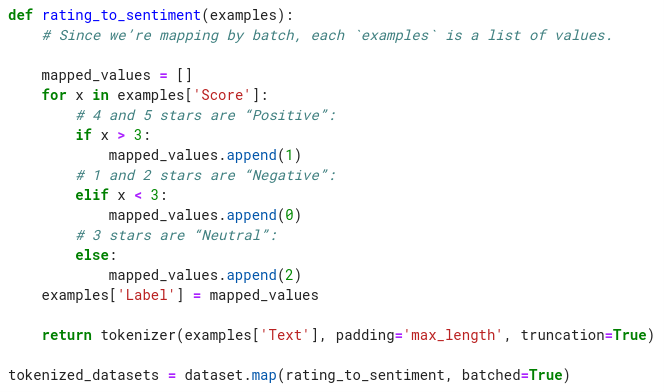
Before we feed our dataset into our model, we also need to tokenize, encode, and pad our text corpus. And for our labels, we would like to transform our star ratings to simply “Positive,” “Negative,” and “Neutral” sentiments. Hugging Face provides us with a tokenizer of its own:

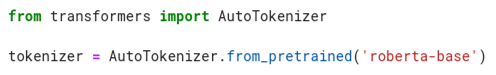
After importing the AutoTokenizer class, we specify the model name (also referred to as “checkpoint”) from the list of model repos on Hugging Face. I chose the RoBERTa base model, which is an improved version of BERT. We then instantiate the tokenizer class from the pre-trained model vocabulary by calling .from_pretrained(). Now, let’s tokenize and remap the star rating to sentiment in a single step using Hugging Face’s famous .map() method:

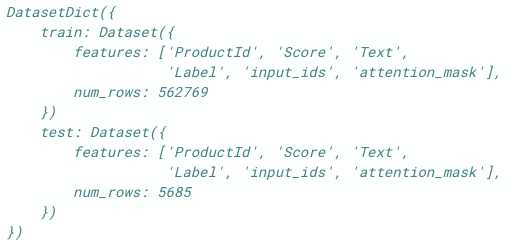
The .map() method accepts a function. Notice also that we specified mapping in batches for improved performance. Inside the mapping function, we created a new dataset key, “Label,” that uses enumerated values for “Positive,” “Negative,” and “Neutral” labels. In the return statement, we call the tokenizer on the “Text” items. Depending on your hardware and the size of the data, it will take a few minutes to finish creating a new dataset object. When it’s complete and we print out the variable, tokenized_datasets, you’ll notice that the object automatically creates several new features: “input_ids,” “token_type_ids,” and “attention_mask,” – which are used for the model training:

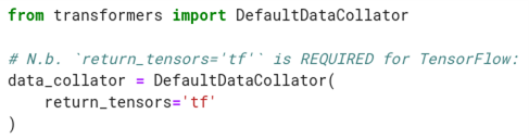
To assemble a list of samples (data) into a training mini-batches, we use “data collators.” Data collators usually pad the mini-batches to be of equal length, and concatenates them into a single tensor; though, depending on the use case, their logic can be far more complex. Let’s instantiate a data collator now:

We then pass our data collator, along with the labels and the features that the tokenizer created into .to_tf_dataset() – this will convert our DatasetDict into a data structure that TensorFlow accepts:

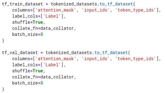
I chose a batch size of 8, but depending on the hardware you’re training on, you may want to choose something else – just remember the batch size number should be a power of two (e.g. 4, 8, 16, 32, 64, etc.).

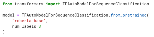
With our dataset now TensorFlow-ready, let’s build our model. Similar to how we instantiated the tokenizer class, we will instantiate the model by calling .from_pretrained(). We will instantiate TFAutoModelForSequenceClassification, which is a generic model class, and set the num_labels argument to 3 since we have 3 label class values (0, 1, 2). This will load the RoBERTa model, along with its (pre-trained) weights:

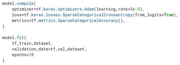
Finally, we compile and train the model, just as we would in TensorFlow:

One detail to pay attention to is that the default learning rate for Adam optimizer is 1e-3; however, we set the learning rate to 5e-5 in our example – this is a much more ideal value for transformer networks like BERT/RoBERTa.

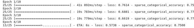
If all is well, when we run model.fit(), we should see the usual Keras progress bar as the model trains:

It is strongly recommended that you have access to (and enable) GPU for training; transformer networks are computationally intensive and take a long time to train – even compared to other deep neural networks – so trying to train our model on CPU would be excruciatingly slow.

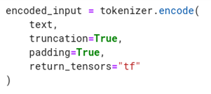
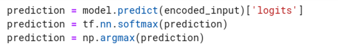
Now that we have retrained the RoBERTa model to our dataset, let’s use it to make predictions. Our prediction function should be able to take an input, a string of text, and apply the same data transformation we applied for training (i.e. tokenize, pad, and encode the input):

With the transformed input, we can feed it into model.predict(); however, the output we get from our model is the “logits” – the values of the last layer of the network, before softmax is applied. We can apply the softmax ourselves and call np.argmax() to get the index of the highest probability, which corresponds to the class categories we defined:

We can make a small improvement to our method by converting the class ids to text labels. The model.config.id2label is a user-definable set of key-value pairs specifically made for this scenario. If our prediction output (after argmax) is 0, we would specify the label value to be “Negative”:

Synthesizing all these points, our prediction function will look like this:

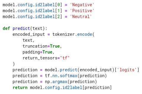
Now, when we call predict(“This is a great product.”), the function returns “Positive.”

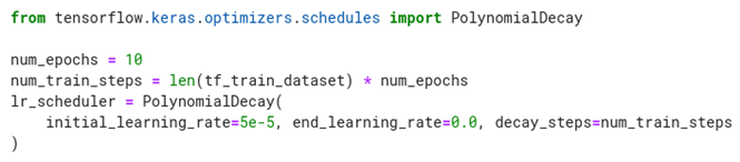
Our model is working OK, but we can optimize it further by using learning rate decay (or “learning rate scheduler,” as Keras/TensorFlow calls it). There are a number of proposed learning rate decay equations/algorithms, but let’s just go with a very simple implementation – this code will tell the training job to start at a learning rate of 5e-5 and slowly decrement to 0 by the end of the training:

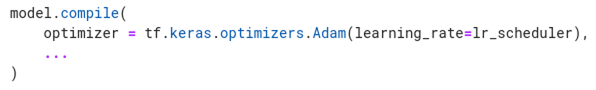
We then pass lr_scheduler to the Adam optimizer inside model.compile:

This wraps up this short tutorial on fine-tuning a Hugging Face model. The benefit of fine-tuning over using Hugging Face’s pipeline function is the ability to adjust hyperparameters for the specific problem we’re trying to solve – as opposed to a model that’s trained on generic corpus of text. We can, of course, fine-tune and apply transfer learning with Keras as well, but with Hugging Face, we can experiment with thousands of different pre-trained checkpoints (models) with ease. And in machine learning, where iterating over new ideas is essential, the ability to do so is an invaluable asset.